On-street parking management
Time-restricted On-street parking management under road congestion
0. Introduction
In unban road networks, the rising demand for on-street parking has intensified drivers’ difficulty in locating available parking spaces while simultaneously aggravating traffic congestion and creating long-standing challenges for transport authorities.
Traditional on-street parking management approaches have primarily emphasized the static construction and allocation of on-parking facilities within urban road networks. However, as urban road networks have reached a state of spatial and functional maturity, large-scale planning and reallocation of on-street parking spaces have become increasingly impractical, constrained by physical limitations, regulatory restrictions, and socioeconomic considerations. Recent research trends in parking management have shifted dynamic pricing strategies and multimodal curb space utilization, yet few research have examined time-restricted parking policies.
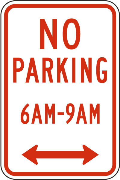
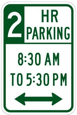
This study develops an optimization framework for spatio-temporal on-street parking management in urban road networks to determine both the road segments and the time periods during which on-street parking restrictions should be implemented, while explicitly accounting for the congestion effects induced by curbside parking activities. The framework captures the interdependence between on-street parking and network performance, enabling more adaptive and congestion-responsive curb management strategies.
1. Problem Statement
On-street parking constitutes a necessary yet scarce infrastructure in urban road networks, where high demand often exceeds limited supply. However, parking activities introduce negative externalities, primarily by reducing effective roadway capacity and increasing delay.
Consider a transport authority seeking to manage this trade-off by imposing on-street parking time restrictions across road segments and time periods. The restrictions directly change travel times on different road segments, thereafter affecting drivers’ route choices and thus the congestion level in the road network. This is because drivers independently select routes that minimize their individual travel time from their origins to destinations, according to wardrop’s principle. The authority’s objective is to satisfy as many parking demand as possible while control the congestion level simultaneously. However, he cannot determine the route choice of drivers directly, but only through the decision of parking restrictions.
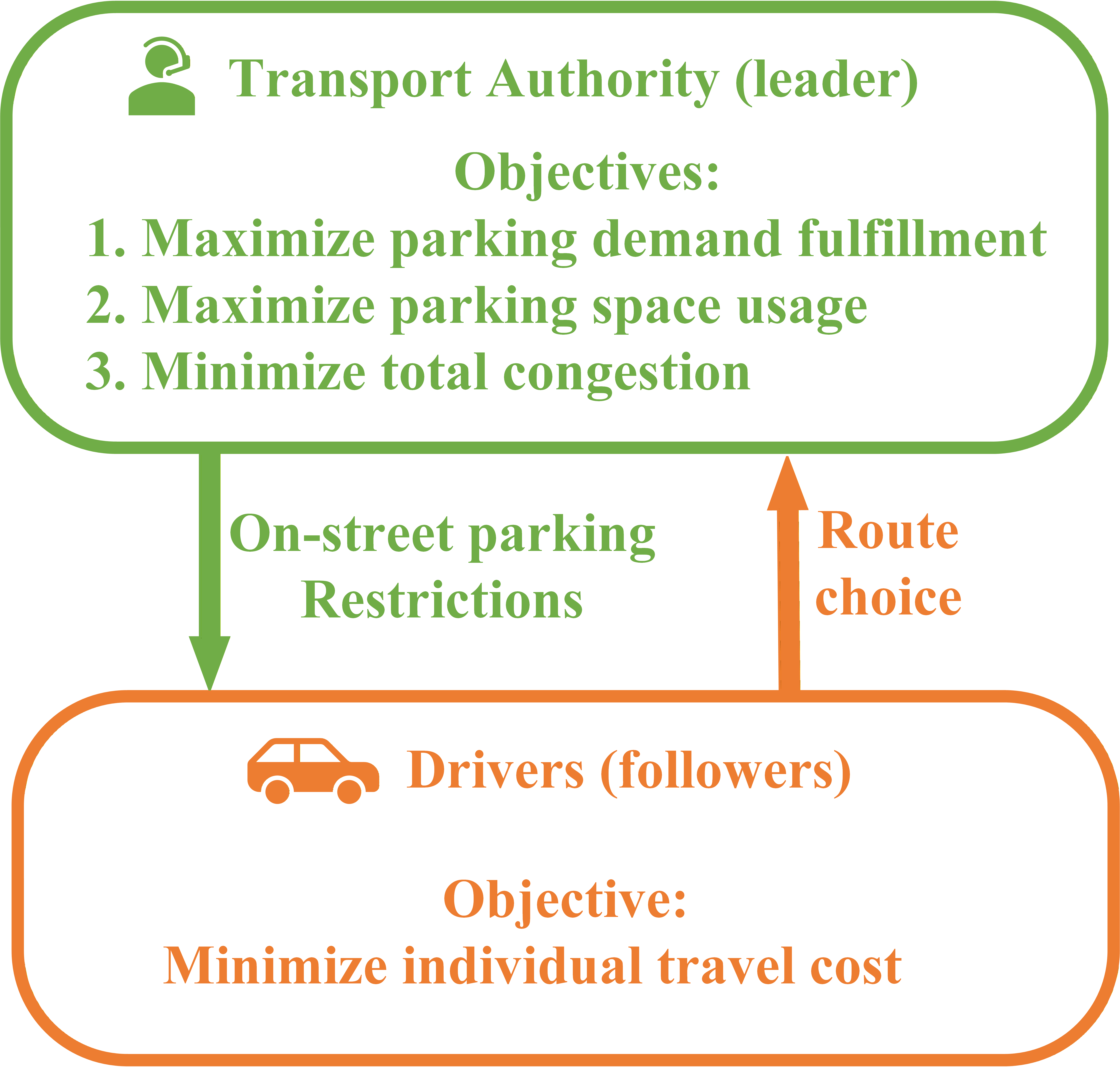
This constitute a stackelberg leader-follower game between the authority and drivers, where the authority acts as the leader and users as the followers. The decision process is modeled as a bi-level discrete network design problem (DNDP), with the upper level representing the authority’s optimization of on-street parking restriction strategies and the lower level representing drivers’ route choice behavior between origin–destination pairs.
1.1 The transport authority’s game
As the leader in the Stackelberg game, the transport authority’s upper-level problem objectives are threefold: (1) minimize unsatisfied parking demand (2) minimize idle on-street parking space numbers, and (3) minimize network congestion, quantified as the Total system travel time.
The authority cannot directly determine the drivers’ route choice. Instead, he indirectly alter drivers’ route choices through the parking restriction policies. The upper-level decision variable are the specific parking restrictions imposed. These policies are designed to be highly granular, allowing for differentiation both spatially (across various road segments) and temporally (across different time periods).
For instance, to mitigate congestion, the authority might enact a strict prohibition on on-street parking within the central business district (CBD) during peak morning and evening hours. Conversely, these restrictions might be relaxed or lifted entirely during off-peak periods or in less congested residential areas to better accommodate local parking demand.


1.2 The impact of on-street parking on road congestion
The negative externalities of on-street parking are quantified by the resulting reduction in effective link capacity $c$. Two link capacity reduction factors are introduced to model capacity reduction level. First, the lane width reduction factor $f_l$, accounting for the physical narrowing of the roadway available to through-traffic; and second, the speed reduction factor $f_p$, which capture disruptive effects and turbulence caused by vehicles maneuvering into and out of parking spaces.


Specifically, the effective link capacity is formulated as: \(c = c_0 f_l f_p\) ,where c_0 is the free flow capacity.
1.3 The drivers’ game
The lower-level problem models the route choice behavior of drivers, where each driver non-cooperatively selects a path to minimize their individual travel time, collectively forming a User Equilibrium (UE) traffic flow pattern. This equilibrium flow is directly influenced by the authority’s parking restrictions, since link travel time is a direct function of the effective link capacity. The travel time $t$ is formulated as:
\[t = t_0 (1 + \alpha (\frac{x}{c_0 f_l f_p})^\beta)\]where $t_0$ denotes free flow time, $\alpha$ and $\beta$ are parameters.
2. Model formulation
Consider a network $G = (N,A)$, where $N$ denotes the set of nodes, $A$ denotes the set of directed links, $A_{0}$ denotes the set of links that do not have curbside parking spaces. Each link $(i,j) \in A$ in $A$ is directional, starting from node $i \in N$ and ending at node $j \in N$. Let $R$ be the set of origin nodes and $S$ be the set of destination nodes, let $RS$ be the set of all origin-destination pairs.
2.1 Upper-level
To capture the dynamic nature of parking activities, the arrival and departure of vehicles at on-street spaces are modeled using queuing theory.
Specifically, consider a road segment with $C$ number of on-street parking spaces, where each parking space represent a server. A server is considered “busy” if the space is occupied by a vehicle and “idle” otherwise. Two standard stochastic assumptions are made:
- The arrival of vehicles follows Poisson distribution with an average rate of $λ$
- The on-street parking duration of vehicles follows exponential distribution with parameter $μ$.
A critical operational constraint of on-street parking is that vehicles are generally not permitted to stop in the middle of a travel lane or drive in reverse to wait for a space. Consequently, there is no waiting queue in this system. If an arriving vehicle finds all $C$ spaces occupied, it cannot wait and is considered “lost” (i.e., it must continue driving). This “no-queue” condition means the total system capacity is equal to the number of servers. Therefore, the on-street parking system on a road segment during a time period can be well modeled as an M/M/C/C queuing system.

The probability that an arriving vehicle finds all $C$ parking spaces occupied, known as the rejection probability $p_c$, is given by the Erlang B formula. And the average number of occupied spaces $o$ is the average customer numbers in the system, given as follows:
\[\begin{align*} & p_{c} = \frac{\frac{(\lambda/\mu)^{C}}{C!}}{\sum_{k=0}^{C} \frac{(\lambda/\mu)^{k}}{k!}} \\ & n = \lambda \cdot (1 - p_c) \end{align*}\]Let $u$ denote the unsatisfied parking demand and $z$ denote idle parking spaces, which are defined as:
\[\begin{align*} & u = \lambda \cdot p_c \\ & z = max\{0, C - n\} \end{align*}\]$u$ and $z$ correspond to the transport authority’s objective (1) minimize unsatisfied parking demand and (2) minimize idle parking space, respectively. The third objective of the authority is the total system travel time, denoted as $\sum x \cdot t(x)$. Thereafter, the upper-level’s objective is formulated as:
\[\min_y \quad F(x, y) = w_1 u + w_2 v + w_3 x \cdot t(x)\]2.2 Lower-level
The lower-level is a User equilibrium traffic assignment problem, formulated as:
\[\begin{align*} \min_x \quad & f(x, y) = \sum_{(i,j) \in A}\int_{0}^{x_{ij}} t_{ij}(u) \, du \\ s.t. \quad & x_{ij} = \sum_{r \in R}x_{ij}^{r}, \quad\forall (i,j) \in A \\ & x_{ij}^{r} \geq 0, \quad \forall (r,s) \in RS, (i,j) \in A \\ & \sum_{i: (k,i) \in A}x_{ki}^{r} - \sum_{j: (j,k) \in A} x_{jk}^{r} = b_{k}^{r}, \quad \forall (r,s) \in RS, \forall k \in N\\ & b_{k}^{r} = \begin{cases} \sum_{s \in S \backslash \{r\}} d_{rs}, \quad k = r \\ -d_{rk}, \quad k \neq r \\ 0, \quad others \end{cases} \label{b_k^rs} \\ \end{align*}\]3. Solution methodology
The proposed discrete network design problem, modeled as a bi-level problem, is mathematically a Non-convex MINLP. It is non-convex due to two reasons: First, the upper-level decision variable is discrete. Second, the lower-level UE equilibrium condition, that is, replacing the lower-level by KKT conditions yields a MPEC.
3.1 Model analysis
The prevailing solution methodology for a Non-linear bi-level programming problem are listed below:
- Heuristics and Metaheuristics. A great many of research paper uses metaheuristics such as evolutionary algorithms, because of the performance of obtaining a high-quality solution in relatively short computation time.
- KKT reformulation and piece-wise linearization. This approach transform the problem into a MPEC, eliminate the equilibrium constraint with big-M and approximate non-linear function with a pice-wise linear function.
- Generalized benders decompotision.
3.2 Lower bound
To find the optimal solution, a strategy of iteratively tighting upper-bound(UB) and lower-bound(LB) is employed. A valid lower bound is obtained by solving a Relaxed Problem (RP). This RP is constructed by removing the lower-level optimality constraint:
Original Problem(OP):
\[\begin{align*} \min_{x,y}\; & F(x,y) \\ \text{s.t.}\; & g(x,y) \le 0, \\ & x \in \arg\min_{u \in X}\; \{\, f(u,y) \mid f(u,y) \le 0 \,\}, \\ & h(x,y) \le 0 . \end{align*}\]Relaxed Problem(RP):
\[\begin{align*} \min_{x,y}\; & F(x,y) \\ \text{s.t.}\; & g(x,y) \le 0, \\ & h(x,y) \le 0 . \end{align*}\]This relaxation transforms the bi-level model into a single-level Mixed-Integer Non-Linear Program (MINLP). The RP can be solved using a method like the extended cutting-plane method. The objective value of the RP’s solution provides a valid lower bound (LB) on the optimal value of the original problem.
3.3 Upper bound and cut generation
Solving the RP yields an upper-level solution $y^k$. This solution is generally not bi-level feasible because its corresponding $x^k$ does not necessarily represent lower-level optimality, namely the user equilibrium flow pattern.
To find a valid upper bound (UB), lower-level User Equilibrium (UE) subproblem is solved with $y^k$ fixed. This yields a feasible UE flow $\tilde{x}$. The pair $(\tilde{x}, y^k)$ is a true feasible solution to the original bi-level problem, and its objective value, $F(\tilde{x}, y^k)$, serves as a valid upper bound. The best UB found so far is stored as the incumbent solution and the lower-level solution is stored in set $\tilde{X}$.
To improve the search, cuts are added to the RP to prune the solution space.
- Optimality cut: After finding a new incumbent UB, an optimality cut is added to the RP.
The cut is added based on the fact that, for any feasible flow $x \in X$ in the lower-level, it must follow UE pattern, which minimize $f(x, y)$ for any given upper-level variable $y$. Therefore, for any explored $\tilde{x} \in X$, any unexplored $x $should have a lower UE cost, or else there is no need to explore the solution in the RP since it is no better than incumbent solutions.
- Exclusion (No-Good) Cut: To prevent the algorithm from re-enumerating the same upper-level decisions, an exclusion cut is added after each iteration. This cut forbids the algorithm from selecting the same set of discrete decisions $y^k$ in future iterations.
4. Numerical Experiments
The model is tested on the LangFang road network, with 78 nodes and 268 links. The roadnetwork is shown as below:
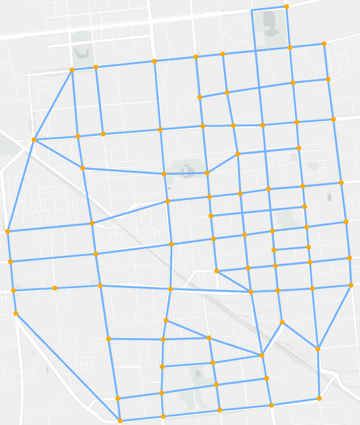
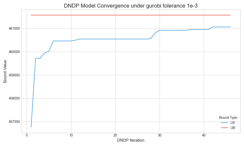
The Termination Gap is set as 0.1% for the Bi-level problem, and 0.01% for frank-wolfe algorithm. It is tested under two gurobi tolerance gap, as shown below:
